Preliminaries of Causal Graphs#
Most existing methodologies for average / heterogeneous treatment effects and personalized decision making rely on a known causal structure. This enables us to locate the right variables to control (e.g., confounders), to intervene (e.g., treatments), and to optimize (e.g., rewards). However, such a convenience is violated in many emerging real applications with unknown causal reasoning. Causal discovery thus attracts more and more attention recently to infer causal structure from data and disentangle the complex relationship among variables.
General Causal Graph Terminology#
Consider a graph \(\mathcal{G} =(\mathbf{Z},\mathbf{E})\) with a node set \(\mathbf{Z}\) and an edge set \(\mathbf{E}\). A node \(Z_i\) is said to be a parent of \(Z_j\) if there is a directed edge from \(Z_i\) to \(Z_j\). Let the set of all parents of node \(Z_j\) in \(\mathcal{G}\) as \(PA_{Z_j} (\mathcal{G})\). A directed graph that does not contain directed cycles is called a directed acyclic graph (DAG). Suppose a DAG \(\mathcal{G}=(\mathbf{Z},\mathbf{E})\) that characterizes the causal relationship among \(|\mathbf{Z}|=d\) nodes, where \(\mathbf{Z}=[Z_1,Z_2,\cdots,Z_d]^\top \) represents a random vector and an edge \(Z_i\rightarrow Z_j\) means that \(Z_i\) is a direct cause of \(Z_j\).
Example 1: Causal Graph for Heterogeneous Treatment Effect and Personalized Decision Making#
In this example, the feature \(S\) determines the treatment assignment \(A\) (i.e., \(S\rightarrow A\)) and the outcome \(R\) (i.e., \(S\rightarrow R\)), and the treatment assignment \(A\) further influences the outcome \(R\) (i.e., \(A\rightarrow R\)).
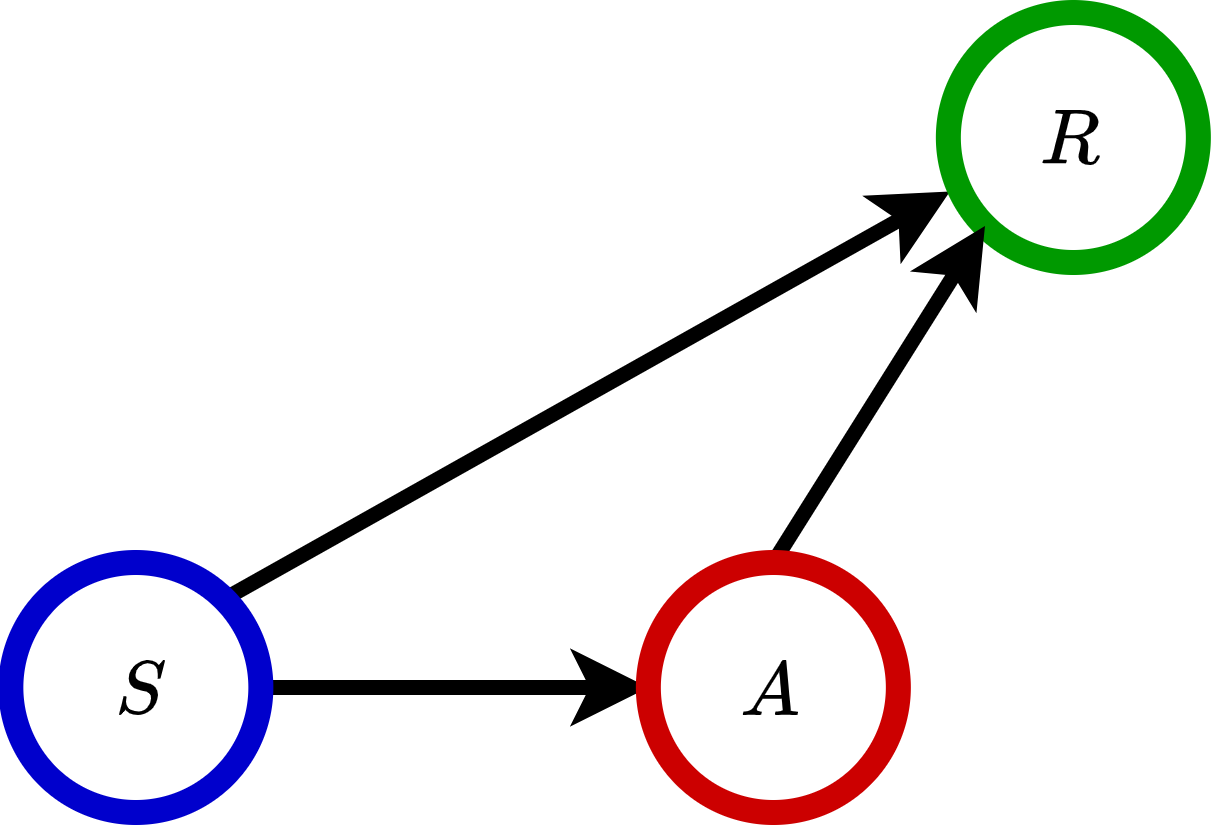
Based on this causal graph, to optimize the outcome of interest, the doctor should assign the right treatment according to different features. Thus, the methods for personalized decision making focus on modeling the conditional mean outcome and the propensity score.
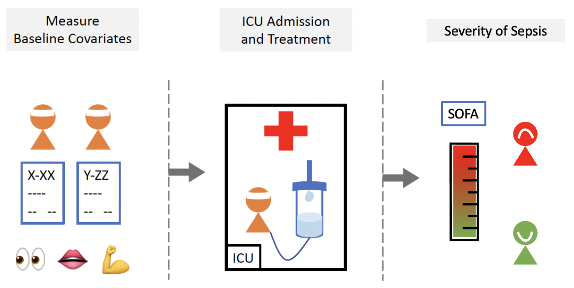
Real Case: Personalized Decision Making in Sepsis for Intensive Care Unit (ICU)#
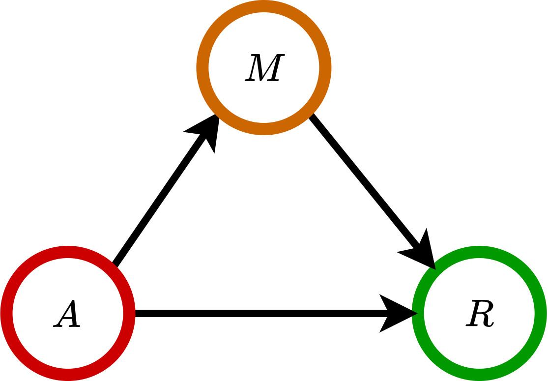
Toy Example 2: Causal Graph for Causal Mediation Analysis#
Causal mediation analysis (CMA) is a method to dissect total effect of a treatment into direct and indirect effect. The direct effect is how the treatment directly affects the outcome, and the indirect effect is transmitted via mediator \(M\) to the outcome.
Pearl et al. (2009) provided a comprehensive review of recent advances in causal mediation analysis using ‘do-operator’ by graphical methods. Let \(\mathbf{M}=[M_1,M_2,\cdots,M_p]^\top \) be mediators with dimension \(p\). Suppose there exists a weighted DAG \(\mathcal{G}=(\mathbf{Z},\mathbf{E})\) that characterizes the causal relationship among \(\mathbf{Z}=[A, \mathbf{M}^\top, R]^\top \). The total effect (\(TE\)), the natural direct effect that is not mediated by mediators (\(DE\)), and the natural indirect effect that is regulated by mediators (\(IE\)) are defined as:
where \(do(A=a)\) is a mathematical operator to simulate physical interventions that hold \(A\) constant as \(a\) while keeping the rest of the model unchanged, which corresponds to remove edges into \(A\) and replace \(A\) by the constant \(a\) in \(\mathcal{G}\). Here, \(\mathbf{m}^{(a)}\) is the value of \(\mathbf{M}\) if setting \(do(A=a)\), and \(\mathbf{m}^{(a+1)}\) is the value of \(\mathbf{M}\) if setting \(do(A=a+1)\). Refer to Pearl et al. (2009) for more details of `do-operator’.
Remarks#
Connection to Average Treatment Effect: When there is no mediator, i.e., only \(A\) and \(Y\) in the system, there is no indirect effect. Then the defined total effect (\(TE\)) reduced to the average treatment effect (ATE): \(\text{ATE} = E[R^*(1) - R^*(0)] = E[ R|do(A=1)] - E[ R|do(A=0)] = TE = DE\).
Connection to Conditional Average Treatment Effect: When there is no mediator but with additional modifiers \(S\) in the system, we have the conditional average treatment effect (CATE), i.e., \(\text{CATE} = E[R^*(1) - R^*(0)|S] = E[ R|do(A=1),S] - E[ R|do(A=0),S] = DE(S) = TE(S)\).
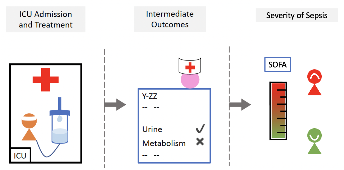
Real Case: Personalized Decision Making in Sepsis for Intensive Care Unit (ICU)#
Toy Example 3: Causal Graph for Mediated Personalized Decision Making#
In this example, the feature \(S\) determines the treatment assignment \(A\) (i.e., \(S\rightarrow A\)), the mediators \(M\) (i.e., \(S\rightarrow M\)), and the outcome \(R\) (i.e., \(S\rightarrow R\)), and the treatment assignment \(A\) further influences the mediators \(M\) (i.e., \(A\rightarrow M\)) and the outcome \(R\) (i.e., \(A\rightarrow R\)). In addition, the mediators \(M\) also affects the outcome \(R\) (i.e., \(M\rightarrow R\)).
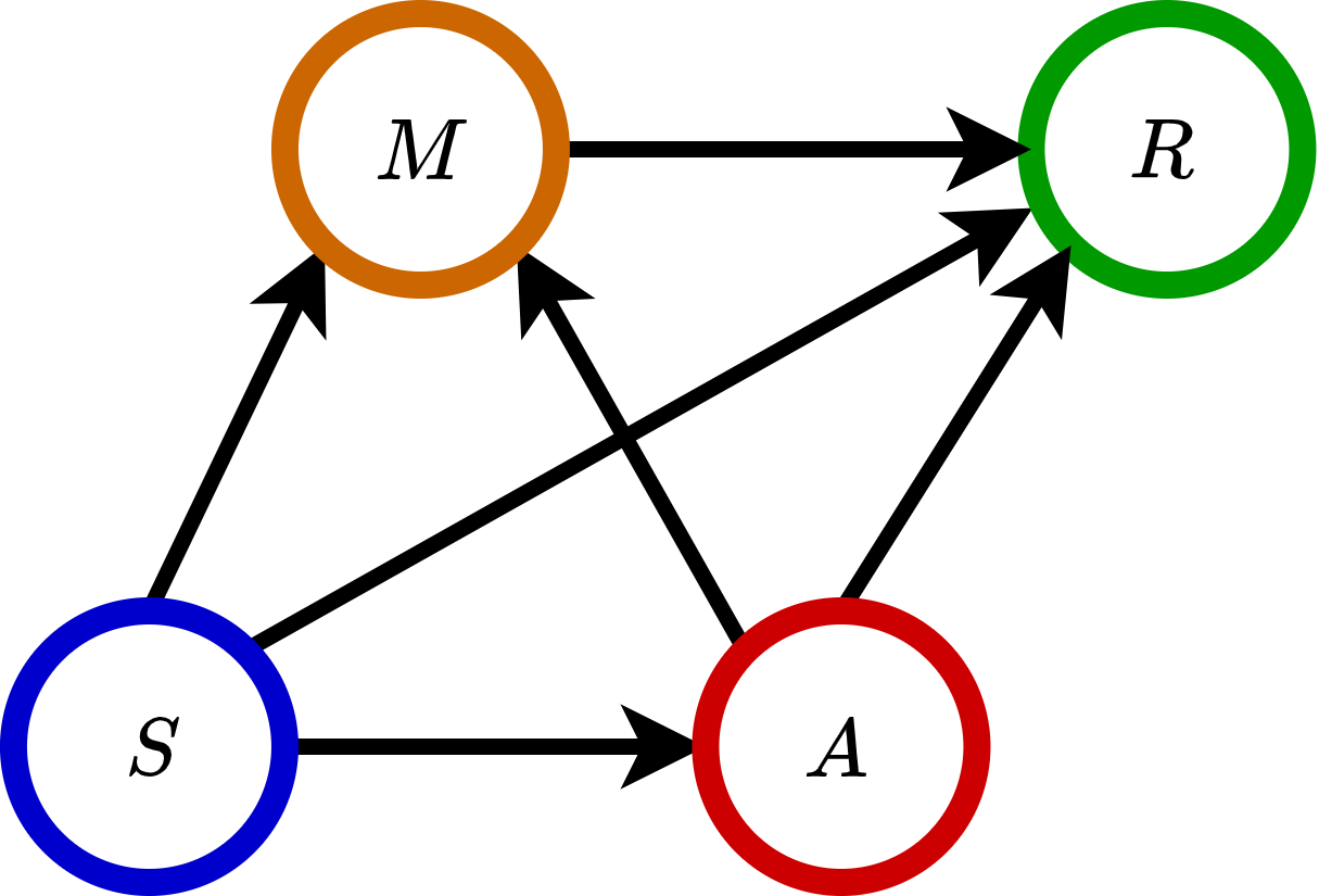
Based on this causal graph, to optimize the outcome of interest, the doctor should assign the right treatment through useful mediators according to different features.
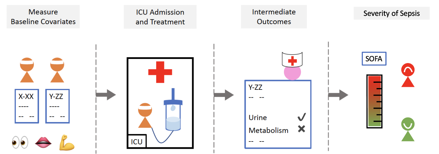
Real Case: Personalized Decision Making in Sepsis for Intensive Care Unit (ICU)#
References#
[1] Judea Pearl et al. Causal inference in statistics: An overview. Statistics surveys, 3:96–146, 2009.
[2] Pater Spirtes, Clark Glymour, Richard Scheines, Stuart Kauffman, Valerio Aimale, and Frank Wimberly. Constructing bayesian network models of gene expression networks from microarray data. 2000.
[3] Markus Kalisch and Peter Bühlmann. Estimating high-dimensional directed acyclic graphs with the pc-algorithm. Journal of Machine Learning Research, 8(Mar):613–636, 2007.
[4] Rajen D Shah and Jonas Peters. The hardness of conditional independence testing and the generalised covariance measure. arXiv preprint arXiv:1804.07203, 2018.
[5] Shohei Shimizu, Patrik O Hoyer, Aapo Hyvärinen, and Antti Kerminen. A linear non-gaussian acyclic model for causal discovery. Journal of Machine Learning Research, 7(Oct):2003–2030, 2006.
[6] Peter Bühlmann, Jonas Peters, Jan Ernest, et al. Cam: Causal additive models, high-dimensional order search and penalized regression. The Annals of Statistics, 42(6):2526–2556, 2014.
[7] David Maxwell Chickering. Optimal structure identification with greedy search. Journal of machine learning research, 3(Nov):507–554, 2002.
[8] Joseph Ramsey, Madelyn Glymour, Ruben Sanchez-Romero, and Clark Glymour. A million variables and more: the fast greedy equivalence search algorithm for learning high-dimensional graphical causal models, with an application to functional magnetic resonance images. International journal of data science and analytics, 3(2):121–129, 2017.
[9] Xun Zheng, Bryon Aragam, Pradeep K Ravikumar, and Eric P Xing. Dags with no tears: Continuous optimization for structure learning. In Advances in Neural Information Processing Systems, pp. 9472–9483, 2018.
[10] Yue Yu, Jie Chen, Tian Gao, and Mo Yu. Dag-gnn: Dag structure learning with graph neural networks. arXiv preprint arXiv:1904.10098, 2019.
[11] Shengyu Zhu and Zhitang Chen. Causal discovery with reinforcement learning. arXiv preprint arXiv:1906.04477, 2019.
[12] Cai, Hengrui, Rui Song, and Wenbin Lu. “ANOCE: Analysis of Causal Effects with Multiple Mediators via Constrained Structural Learning.” International Conference on Learning Representations. 2020.